Stock Market Gap Phenomenon Analysis
Stock Market Gap Phenomenon Analysis using Statistical Techniques
Introduction
What is a Price Gap in stock market?
A gap is an area of discontinuity in a security’s chart where its price either rises or falls from the previous day’s close with no trading occurring in between. Gaps occur when a security’s price jumps between two trading periods, skipping over a range of prices.
The underlying reasons for gaps are certain significant events (i.e. financial reports, earnings releases, natural disasters or catastrophes, changes in executive management, etc.). These events draw a lot of attention from many investors and generate intense trading activity; therefore, they supposedly represent behavioral patterns of a large group of people.
This project is an attempt to explore the price gap phenomenon on US Stocks, identify relevant parameters, correlations and/or causative relationships.
Data
One of the major challenges that we encountered while trying to get historical constituents that were part of the S&P 500 stock index is the dataset which is survivorship bias free.
The historical S&P 500 constituents dataset was found here. The original list is a download associated with the book Trading Evolved. S&P 500 Historical Components & Changes.csv is the original file that runs from 1996 to 2019. Every couple of months, S&P 500 Wikipedia page is used to update sp500_changes_since_2019.csv with any changes that have occurred to the index.
The ticker names are correct on any day you pick from the csv file and all of these ticker names are unique. If they are missing later, we can assume they were removed from the index and you sell that position. Even if the company was not removed but the symbol changed, It means the company got acquired. The algorithm will pick up the new name if it meets your criteria.
The historical S&P 500 constituents file is later processed and the information extracted is stored in a dictionary with constituent ticker as the key and its corresponding time frames of its presence in the stock index as values. Later, the dictionary is further iterated over and the required data is downloaded from the yahoo finance for their respective time frames and the data for each ticker is compiled and stored in individual files.
Data Selection
Once we have the dictionary with tickers and their respective timeframes, The historical stock data for each of those tickers is downloaded from the public source yahoo finance. Apart from the tickers that we have listed in the dictionary with timeframes we will also need the historical data of the stock GSPC which is the stock representing the S&P 500 stock index.
Each of the files that we created in our previous step has EOD stocks historical data such as open, close, high, low, volume and adjusted. However a lot of this data has to be further carefully analyzed and cleaned before proceeding with the modeling.
Data Preparation
Our dataset sums upto around 600 csv files with EOD data for each stock. However we have to calculate a few more metrics using the existing EOD metrics to use them as features in the data analysis process. Let’s go step by step:
- Removing files with minimal data: For our data analysis step we need at least 10 days of EOD data before and after the occurrence of the gap. So, we remove files having less than 25 rows.
- Removing rows with na values: Some of the rows in the dataset have na values for the EOD stock metrics. Having such values is not going to help us in calculating other relative metrics using the existing ones. Hence rows with na values will be removed.
- Removing files with no data: Some of the downloaded files are empty, therefore such files will be omitted from the collection of datasets for each ticker.
Once the cleaning part is complete we will now proceed with calculating some of the metrics listed below along with their formulas and add them to the same file and save them as ticker_preprocessed.csv under the preprocessed_data folder.
-
Gap type and Gap Size: Gap type is of two types i.e. UP and DOWN. Gap type and Gap size is calculated using the following formulas.
-
Gap Up Size = (Low for Gap day - High for Previous Day) / High for Previous Day
-
Gap Down Size = (High for Gap Day - Low for Previous day) / Low for Previous Day
-
-
Volume Change: The change in volume is calculated using today’s and yesterday’s volume using the following formula.
- Volume Change = (Today’s volume - Yesterday’s volume) / Yesterday’s volume
-
Overnight returns: Is calculated using today’s adjusted close and yesterday’s adjusted close.
- Overnight returns = (Today’s adjusted close - Yesterday’s adjusted close) / Yesterday’s adjusted close
-
Relative daily price range: Is calculated using daily high and low.
- Daily Range = (High for the day - Low for the day) / Low for the day
-
Day of the week and month: We need to extract day of the week and month as potential features.
-
Candle body metric: Is calculated using day close and open using the following formula
- Candle Body Metric = (Today’s close - Today’s open) / Today’s open
-
Adding lag and leads: The following features (“vol_change”, “return”, “adjusted_return”, “range”, “weekday”, “month”, “candle_body_metric”) are calculated for ten days before and after the gap day and saving it to the same gap day row as different features.
Data Analysis
Once the data was collected, pre-processed and cleaned, we ended up with a substantial set of gap observations. Total number of gaps detected was 117207, gaps UP: 64130 or 54.72% and gaps DOWN: 53077 (45.28%).
One of the potential predictors is the day of the week on which the gap has occurred. Therefore, it was interesting to see how gaps are distributed through the weekdays. The following table is the summary of such analysis:
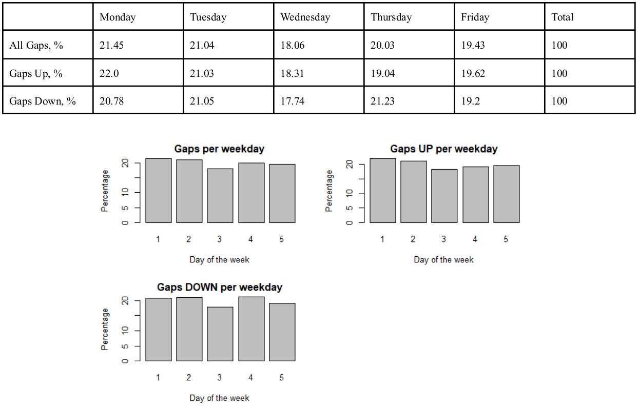
As it can be noted, considerably less gaps of all types occur on Wednesdays. Monday, Tuesday and Thursday are the most productive days for gaps.
Similar motivation applies to the months of the year. Therefore, the statistics for months are shown below.
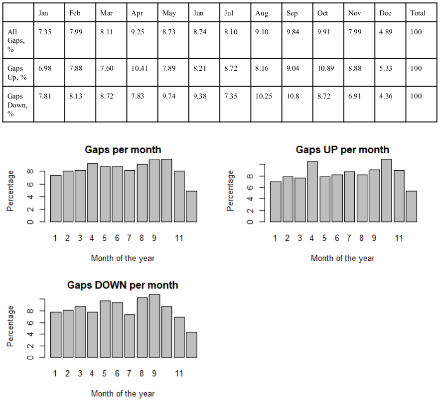
Overall, the last two months of the year are less productive on gaps, as well as July and September, October are the most productive months. Gaps up have spikes in April and October and Gaps down are more frequent May, June and August, September.
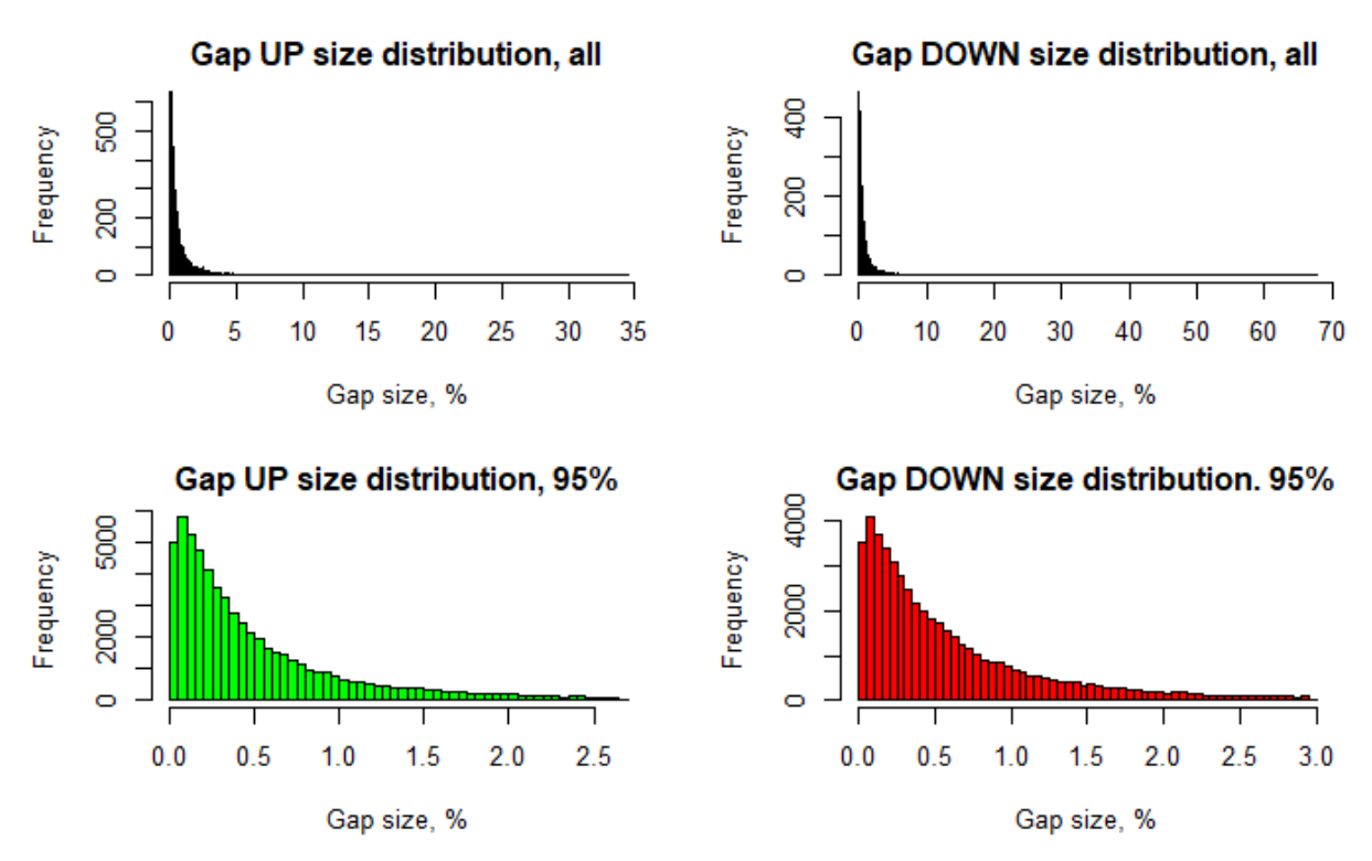
Next question we wanted to answer is how Gaps are distributed by size. The following figure demonstrates the distribution of gap size. The distributions have few very far outliers which will be candidates for removal from the dataset. The distributions for the remaining 95% of the population are shown in the lower row. As we can see the majority of the gaps have size smaller than 3%. We will consider gap size as a predictor.
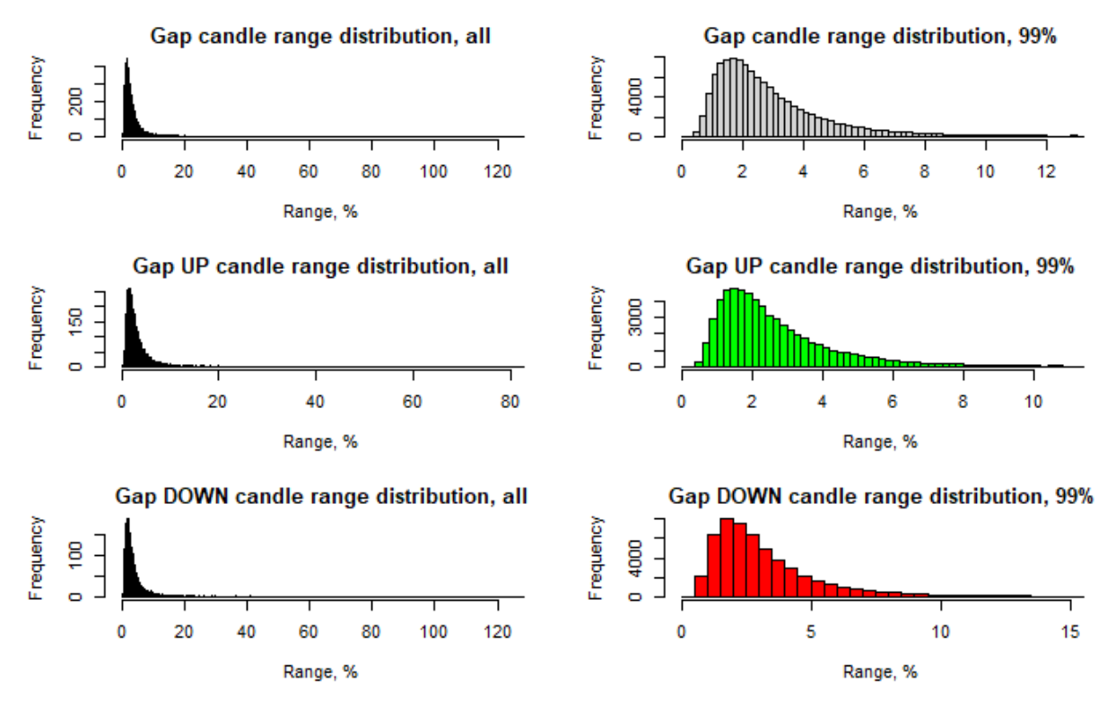
Another feature of the stock price is the relative daily price range which we would like to consider as a predictor. Similar to the gap size the daily range has a small number of very far outliers. The distribution of the remaining 99% of the daily range population is shown on the right side of the picture below. The majority of the daily ranges lay within 12%. And the most common range is between 1 and 2%.
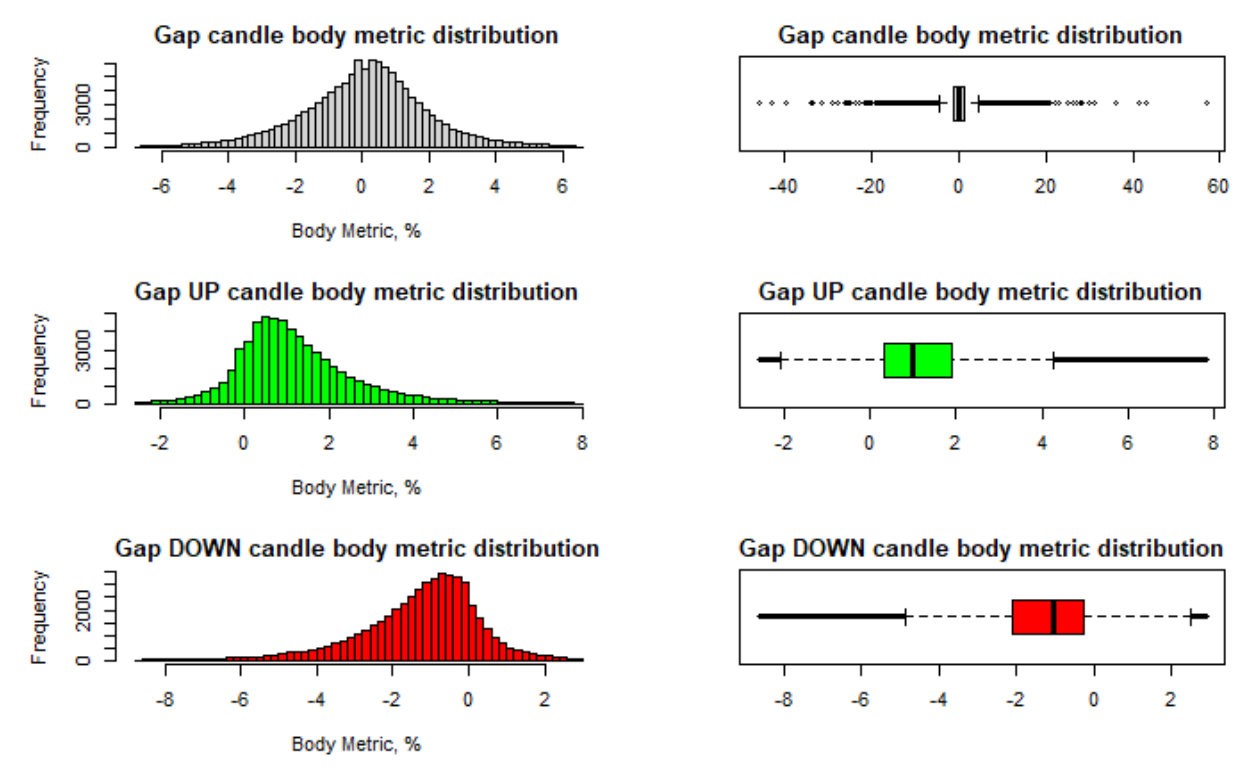
In the context of historical stock prices it is important to preserve the basic dynamics of the prices during the time span. That is why for each time span the prices are represented by multiple values - Open, Close, Low, High and Adjusted prices. In order to capture the dynamics (i.e. Close is higher or lower then Open) and to unbound the prices from the absolute values, we introduced the so called Candle Body Metric. The formula to calculate it was provided earlier in the report. Negative value of this metric will represent the time period when price has fallen and the positive when it has risen. The absolute value of the metric will indicate the amount of the change in prices. The distribution of this newly introduced metric is shown in the picture below. As we can see, the distributions are skewed in opposite directions for gaps Ups and Downs. And the most common difference between Open and Close prices is a little less than 1%.
As we captured multiple variables that may have influence on future returns of the stock, it would be beneficial to explore how they are correlated. The total number of numeric variables is 46. They include a one day ahead return as the output we are trying to predict, gap size, the current and lagged (up to 10 days) variables such as change in trade volume, return, candle body metric, and range. The correlation analysis was performed and several significant findings were noted:
- The Returns are strongly correlated with Candle Body Metric. This makes sense as most often overnight returns are strongly correlated with daily returns. We will keep it in mind as potentially it may suggest removal of irrelevant predictors.
- The Returns are strongly correlated with the size of the Gap. This makes sense too, however the size of the gap may represent not just a change in the price but the influence of significant forces moving the price.
- The daily price ranges have significant autocorrelation.
- Most of the variables have insignificant and very short autocorrelation effects (1-2 days) with the exception of daily price range. This information might be useful in attempting to narrow down the size of the lag considered in time series related regression model or recurrent neural network architecture.
Conclusion and Future Work
During the course of this project we were able to identify and obtain stocks prices data historically belonging to the S & P 500 index. We learned about time series and about survival bias in financial markets. Based on availability of historical data we were able to partially remove survival bias from the collected data. Data cleanup and preprocessing was performed in order to prepare a dataset for data analysis.
Our ultimate goal was to justify, architect, implement and evaluate performance of the recurrent neural network based on LSTM elements. However, it was difficult to reach this goal due to a lot of obstacles encountered while collecting data.
Future recommendations and requirements:
- Obtain more complete data, specifically for the stocks of the companies that were in the S&P 500 index for the period of our interest but delisted or ceased to exist.
- Implement Recurrent Network Architecture and evaluate its performance.
- If successful with RNN, extend it to predict returns for more than one days ahead.