Diabetes Prediction System

Introduction

Diabetes possesses a major cause for blindness, kidney failure, lower-limb amputation, heart attack and stroke. Although diabetes disease has been identified as the most chronic disease across the world, it is the most preventable one at the same time. A healthy lifestyle (primary prevention) and timely diagnosis (secondary prevention) are two main elements of diabetes control.

Machine learning has numerous objectives. Regression, classification, and clustering are the most prevalent. It is also important to introduce Parametric and Non-Parametric Machine Learning Models. Parametric models require specification of certain parameters in order for the model to train and produce results. On the other hand non-parametric models do not require any kind of parametric specifications and can train on the model.

This project applied 5 Linear Regression techniques to predict the presence of diabetes in a person.

Data

The first step of our project work was determining the right data set. Many online resources exist with access to a plethora of classification datasets. We came across many platforms like datahack and dataworld. I selected the Pima Indians Diabetes dataset collected by the National Institute of Diabetes and Digestive and Kidney Diseases for our project.

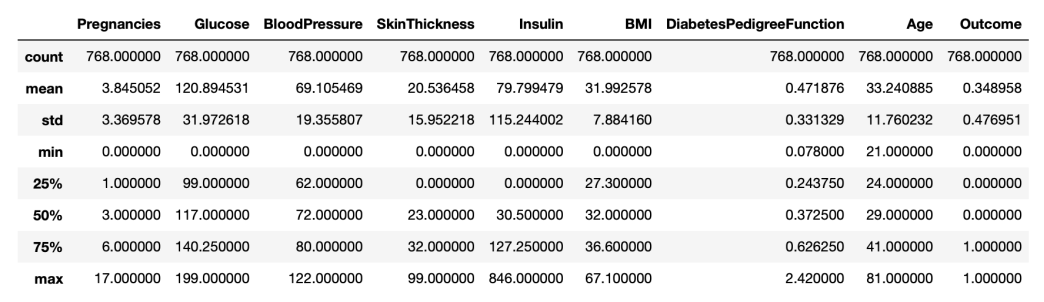
The dataset contains 768 records against 9 attributes i.e. Pregnancies, Glucose, BloodPressure, SkinThickness, Insulin, BMI, DiabetesPedigreeFunction, Age and Outcome. 80% of the dataset was used for training and the remaining 20% was used for testing the trained model.

The 9 columns of the dataset and what each column represents:

• Pregnancies: ​ Number of times pregnant
• Glucose: Plasma glucose concentration a 2 hours in an oral glucose tolerance test
• BloodPressure: Diastolic blood pressure (mm Hg)
• SkinThickness: Triceps skin fold thickness (mm)
• Insulin: 2-Hour serum insulin (mu U/ml)
• BMI: Body mass index (weight in kg/(height in m)^2)
• DiabetesPedigreeFunction: It provides information about diabetes history in relatives and genetic relationship of those relatives with individuals.
• Age: Age (years)
• Outcome: Target

The goal is to predict the Outcome target variable whether a person has a chance of having diabetes or not. The main technical challenge it poses to predicting Outcome is the high frequency of null values in data as it’s medical data so those null values are crucial for out analysis. The goal of this analysis is to solve this issue by a detailed data exploration and cleaning followed by choosing a suitable machine-learning algorithm.

Machine Learning Models

We will deploy 5 linear machine learning algorithms to predict the occurrence of diabetes disease.

Linear Regression

Linear regression makes an attempt to describe the relationship between two variables by analyzing the data and fitting a linear equation to it. Target is seen as a dependent variable, whereas Feature variables are thought to be explanatory factors.

A linear regression line has an equation of the form Y = a + bX, where X is the independent variable and Y is the dependent response variable. The slope of the line is b, and a is the intercept (the value of y when x = 0).

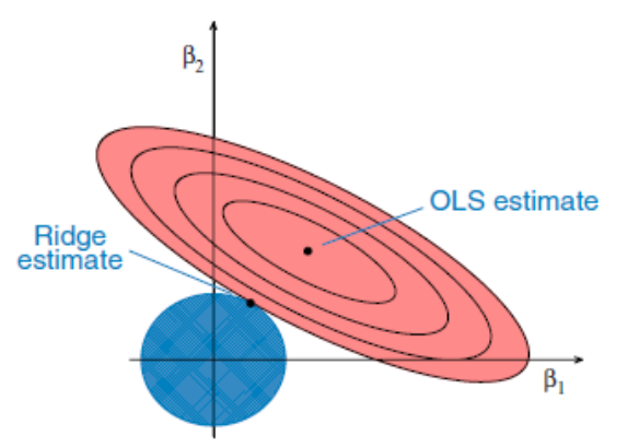
Ridge Regression

Any data that suffers with multicollinearity is analyzed using the model tuning technique known as ridge regression. This technique carries out L2 regularization. Predicted values differ much from real values when the problem of multicollinearity arises, least-squares are unbiased, and variances are significant. The ridge regression cost function is:

λ (lambda) given here is denoted by an alpha parameter in the ridge function, It is also called the penalty term. So, by changing the values of alpha, we are controlling the penalty term. The bigger the penalty, higher is the value of alpha and therefore the magnitude of coefficients is reduced.

Lasso Regression

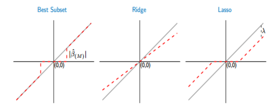
The lasso causes L1 shrinkage, resulting in “corners” in the constraint, which is equivalent to a diamond in two dimensions. If the squared sum “hits” one of these corners, the axis-specific coefficient is reduced to zero. Since the multidimensional diamond has more corners as p rises, it is very likely that some of the coefficients will be set to zero. Thus, shrinkage and (essentially) subset selection are performed via the lasso.

Lasso performs a soft thresholding in contrast to subset selection. The sample path of the estimates moves continuously to zero as the smoothing parameter is varied.

Best Subset Selection

Let’s say we have a set of variables we can use to predict an important event, and we want to select the subset of those variables that most closely matches the outcome. One method is to fit all the potential variable combinations and select the one that meets the best criterion in accordance with specified criteria once we have chosen the type of model (logistic regression, for example). Best subset selection is what we term this.

It takes a lot of calculation to use this method. We need to fit 2^p models when there are 𝑝 possible predictors. Additionally, the issue becomes insurmountable very fast if we want to apply cross-validation to assess their performance. The leaps and bounds technique expedites the process of finding the “best” models and does not necessitate fitting each model individually. In any event, if there are too many predictors, even this technique is useless.

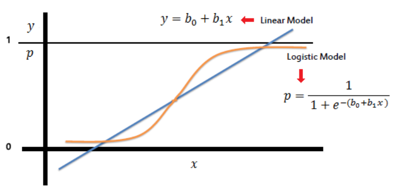
Logistic Regression

Logistic regression is a classification procedure that is used to forecast the likelihood of a target variable. The target or dependent variable has a dichotomous character, which means there are only two potential classes. The representation for logistic regression is an equation. To anticipate an output value, input data are linearly mixed with coefficient values. The output value is represented as a binary value, which distinguishes it from linear regression.

Data Exploration

Visualizations are performed in each step, in order to highlight new insights about the underlying patterns and relationships contained within the data. Here is a list of statistics for each feature.

From the below graph we can say that less than half of the females are suffering from Diabetes Disease with a percentage of 34.9%. Some features contain 0 in the data. It doesn’t make sense here because there is and this indicates that there are missing values in our data. By further looking into the data, we found that it is because there are a number of factors involved in the data to correctly assess the occurrence of diabetes, one of them being the Glucose feature.

Let’s get some more insights about the features with box plots.

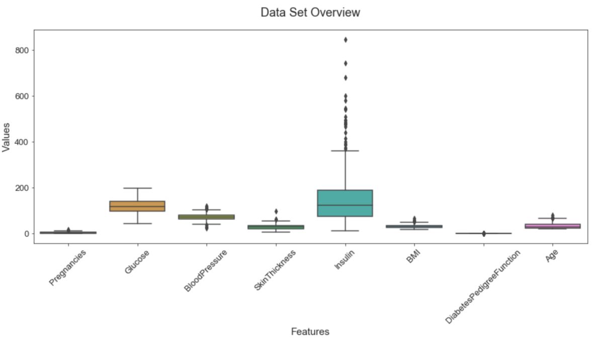
From the above plot we can see that there are outliers in the data and those outliers might be valid values so we can’t replace the missing values with the mean instead we will use the median by target to replace the missing data to get a much more realistic data.

Feature Analysis

For Plasma glucose concentration in 2 hours in an oral glucose tolerance test we got 107 Plasma glucose concentration level for non diabetic females and 140 for diabetic females. For Diastolic blood pressure (mm Hg) we got 70 Diastolic blood pressure for non diabetic females and 74.5 for diabetic females. For Triceps skin fold thickness (mm) we got 27 Triceps skinfold thickness for non diabetic females and 32 for diabetic females. For 2-Hour serum insulin (mu U/ml) we got 102.5 serum insulin for non diabetic females and 169.5 for diabetic females and for Body mass index (weight in kg/(height in m)^2) we got 30.1 Body mass index for non diabetic females and 34.3 for diabetic females.

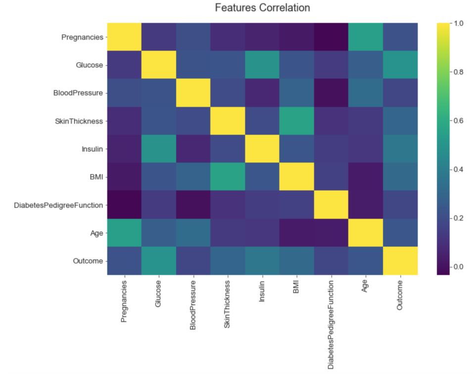
From the above correlation graph we can see that highly correlated features are Pregnancies vs Age, Glucose vs Insulin and SkinThickness vs BMI.

Healthy females are concentrated with 𝐴𝑔𝑒 <= 30 , 𝑃𝑟𝑒𝑔𝑛𝑎𝑛𝑐𝑖𝑒𝑠 <= 6 , 𝐼𝑛𝑠𝑢𝑙𝑖𝑛 < 200 , 𝐺𝑙𝑢𝑐𝑜𝑠𝑒 <= 120 , 𝐵𝑀𝐼 <= 30 , and 𝐵𝑀𝐼 <= 30 and 𝑆𝑘𝑖𝑛𝑇ℎ𝑖𝑐𝑘𝑛𝑒𝑠𝑠 <= 20 .

Conclusion

Results were compiled and visualized, Linear model results were as follows:

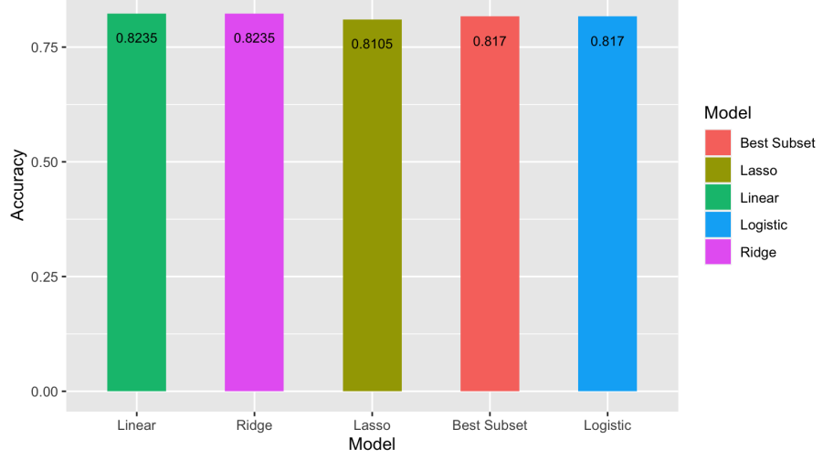
The goal was to predict whether a person has a chance of having diabetes in future. Linear Regression, Ridge Regression, Lasso Regression, Best Subset Selection and Logistic Regression models were trained. Results show that Linear & Ridge Regression achieved the highest accuracy of 82.35% after training, which is very promising considering the small size of available data.

Since we were using linear models on the data we specified a cutoff for calculating our model accuracies which has to be from 0-1 as our Outcome can either be 0 or 1. The models’ accuracies change when we alter the cutoff value. We can see that even Linear Regression and Ridge Regression have the same accuracy based on a cutoff of 0.4. Linear Regression worked best based on the average of the accuracies obtained from altering the cutoff value so “Linear Regression” is selected due to its highest accuracy. The results compiled after the implementation of this algorithm are displayed as above.

The Linear models gave us very positive results considering the size of the data. For future work if we use classification algorithms such as Random Forest, Decision Tree and Support Vector Machine, they will definitely give us better results and we can further test our models by calculating their average accuracy using k-fold cross validation technique.